隨機采樣和隨機模擬：吉布斯采樣Gibbs Sampling實現文檔分類

http://blog.csdn.net/pipisorry/article/details/51525308

吉布斯采樣的實現問題

本文主要說明如何通過吉布斯采樣進行文檔分類（聚類），固然更復雜的實現可以看看吉布斯采樣是如何采樣LDA主題散布的[主題模型TopicModel：隱含狄利克雷散布LDA]。

關于吉布斯采樣的介紹文章都停止在吉布斯采樣的詳細描寫上，如隨機采樣和隨機摹擬：吉布斯采樣Gibbs Sampling(why)但并沒有說明吉布斯采樣到底如何實現的(how)？

也就是具體怎樣實現從下面這個公式采樣？

怎樣在模型中處理連續參數問題？

怎樣生成終究我們感興趣的公式的期望值，而不是僅僅做T次隨機游走？

下面介紹如作甚樸素貝葉斯Na ??ve Bayes[幾率圖模型：貝葉斯網絡與樸素貝葉斯網絡]構建1個吉布斯采樣器，其中包括兩大問題：如何利用共軛先驗？如何通過等式14的條件中進行實際的幾率采樣？

皮皮blog

樸素貝葉斯模型的吉布斯采樣器

問題

基于樸素貝葉斯框架，通過吉布斯采樣對文檔進行（無監督和有監督）分類。假定features是文檔下的詞，我們要預測的是doc-level的文檔分類標簽（sentiment label），值為0或1。

首先在無監督數據上進行樸素貝葉斯的采樣，對監督數據的簡化會在后面說明。

Following Pedersen [T. Pedersen. Knowledge lean word sense disambiguation. In AAAI/IAAI, page 814, 1997.,    T. Pedersen. Learning Probabilistic Models of Word Sense Disambiguation. PhD thesis, Southern Methodist University, 1998. http://arxiv.org/abs/0707.3972.], we’re going to describe the Gibbs sampler in a completely unsupervised setting where no labels at all are provided as training data.

模型表示

樸素貝葉斯模型對應的plate-diagram：

   

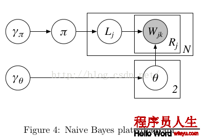
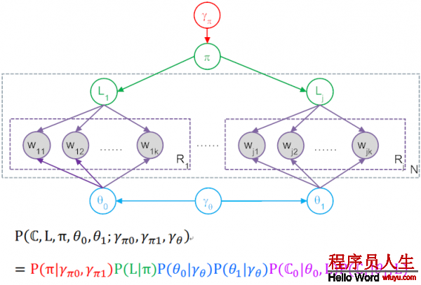
                                                                                                                                                                                         Figure4⑴

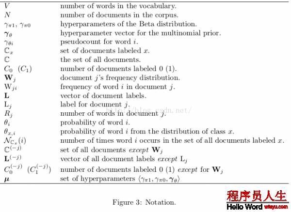
變量代表的意思以下表：

1.每個文檔有1個Label(j)，是文檔的class，同時θ0和θ1是和Lj對應的，如果Lj=1則對應的就是θ1

3.在這個model中，Gibbs Sampling所謂的P(Z)，就是產生圖中這全部數據集的聯合幾率，也就是產生這N個文檔整體聯合幾率，還要算上包括超參γ產生具體π和 θ的幾率。所以最后得到了上圖中表達式與對應色采。

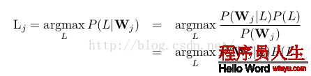
給定文檔，我們要選擇文檔的label L使下面的幾率越大：

文檔生成進程

文檔j的label生成

文檔j的詞袋生成描寫

先驗Priors

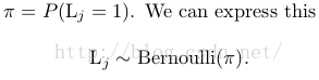
π來自哪里？

hyperparameters : parameters of a prior, which is itself used to pick parameters of the model.

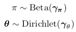
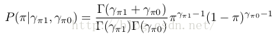
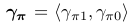
Our generative story is going to assume that before this whole process began, we also picked π randomly. Specifically we’ll assume that π is sampled from a Beta distribution with parameters γ π1 and γ π0 .

In Figure 4 we represent these two hyperparameters as a single two-dimensional vector γ π = γ π1 , γ π0 . When γ π1 = γ π0 = 1, Beta(γ π1 , γ π0 ) is just a uniform distribution, which means that any value for π is equally likely. For this reason we call Beta(1, 1) an “uninformed prior”.

θ 0 和 θ 1來自哪里？

Let γ θ be a V -dimensional vector where the value of every dimension equals 1. If θ0 is sampled from Dirichlet(γθ ), every probability distribution over words will be equally likely. Similarly, we’ll assume θ 1 is sampled from Dirichlet(γ θ ).

Note: θ0為label為0的文檔中詞的幾率散布；θ1為label為1的文檔中詞的幾率散布。θ0and θ1are sampled separately. There’s no assumption that they are related to each other at all.

2.3 模型的狀態空間和初始化

狀態空間

樸素貝葉斯模型中狀態空間的變量定義

? one scalar-valued variable π （文檔j的label為1的幾率）
? two vector-valued variables, θ 0 and θ 1
? binary label variables L, one for each of the N documents
We also have one vector variable W j for each of the N documents, but these are observed variables, i.e.their values are already known (and which is why W jk is shaded in Figure 4).

初始化

Pick a value π by sampling from the Beta(γ π1 , γ π0 ) distribution. sample出文檔j的label為1的幾率，也就知道了文檔j的label的bernoulli幾率散布(π, 1-π)。

Then, for each j, flip a coin with success probability π, and assign label L j(0)— that is, the label of document j at the 0 th iteration – based on the outcome of the coin flip. 通過上步得到的bernoulli散布sample出文檔的label。

Similarly,you also need to initialize θ 0 and θ 1 by sampling from Dirichlet(γ θ ).

派生聯合散布

for each iteration t = 1 . . . T of sampling, we update every variable defining the state space by sampling from its conditional distribution given the other variables, as described in equation (14).

處理進程：

? We will define the joint distribution of all the variables, corresponding to the numerator in (14).
? We simplify our expression for the joint distribution.
? We use our final expression of the joint distribution to define how to sample from the conditional distribution in (14).
? We give the final form of the sampler as pseudocode.

聯合散布的表示和簡化

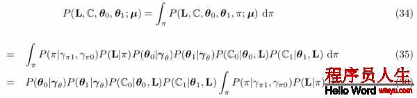
模型對全部文檔集的聯合散布為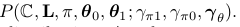

Note： 分號右側是聯合散布的參數，也就是說分號左側的變量是被右側的超參數條件住的。

聯合散布可分解為（通過圖模型）：

因子1：

也即Figure4⑴紅色部份：這個是從beta散布sample出1個伯努利散布，伯努利散布只有1個參數就是π，不要normalization項（要求的是全部聯合幾率，所以在這里糾結normalization是沒有用的），得到：

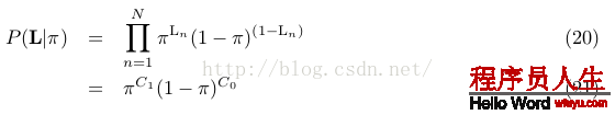
因子2：

也即Figure4⑴綠色部份：這里L是1全部向量，其中值為0的有C0個，值為1的有C1個，屢次伯努利散布就是2項散布啦，因此：

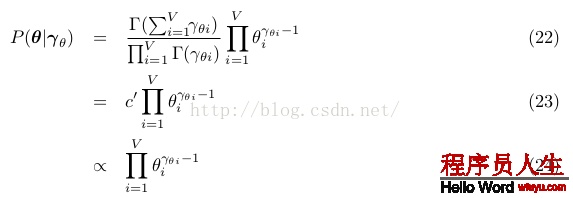
因子3：

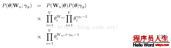
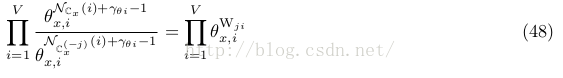
詞的散布幾率，也即Figure4⑴藍色部份：對0類和1類的兩個θ都采樣自參數為γθ的狄利克雷散布，注意所有這些都是向量，有V維，每維度對應1個Word。根據狄利克雷的PDF得到以下表達式，其實這個表達式有兩個，分別為θ0和θ1用相同的式子采樣：

因子4：

P (C 0 |θ 0 , L) and P (C 1 |θ 1 , L): the probabilities of generating the contents of the bags of words in each of the two document classes.

也即Figure4⑴紫色部份：首先要求對單唯一個文檔n，產生所有word也就是Wn的幾率。假定對某個文檔，θ=(0.2,0.5,0.3)，意思就是word1產生幾率0.2，word2產生幾率0.5，假設這個文檔里word1有2個，word2有3個，word3有2個，則這個文檔的產生幾率就是(0.2*0.2)*(0.5*0.5*0.5)*(0.3*0.3)。所以依照這個道理，1個文檔全部聯合幾率以下：

let θ = θ L n:

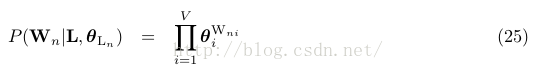
Wni: W n中詞i的頻數。

文檔間相互獨立，同1個class中的文檔合并，上面這個幾率是針對單個文檔而言的，把所有文檔的這些幾率乘起來，就得到了Figure4⑴紫色部份：

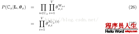
Note: 其中x的取值可以是0或1，所以Cx可以是C0或C1，當x=0時，n∈Cx的意思就是對所有class 0中的文檔，然后對這些文檔中每個word i，word i在該文檔中出現Wni次，求θ0,i的Wni次方，所有這些乘起來就是紫色部份。后式27是規約后得到的結果，NCx (i) ：word i在 documents with class label x中的計數，如NC0(i)的意思就是word i出現在calss為0的所有文檔中的總數，同理對NC1(i)。

聯合散布的表示和先驗選擇的緣由

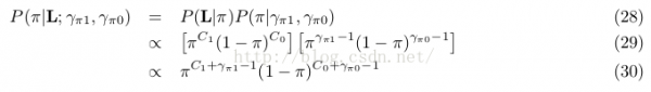
使用式19和21：

使用式24和25：

如果使用所有文檔的詞（也就是使用式24和27）

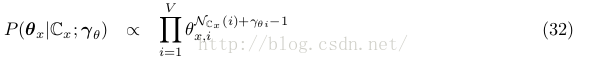
可知后驗散布式30是1個unnormalized Beta distribution, with parameters C 1 + γ π1 and C 0 + γ π0 ,且式32是1個unnormalized Dirichlet distribution, with parameter vector N C x (i) + γ θi for 1 ≤ i ≤ V .

也就是說先驗和后驗散布是1種情勢，這樣Beta distribution是binomial (and Bernoulli)散布的共軛先驗，Dirichlet散布是多項式multinomial散布的共軛先驗。
而超參數就如視察到的證據，是1個偽計數pseudocounts。

讓，全部文檔集的聯合散布表示為：

將隱含變量π積出

why: 為了方便，可以對隱含變量π進行積分，最后到達消去這個變量的目的。我們可以通過積分掉π來減少模型有效的參數個數。This has the effect of taking all possible values of π into account in our sampler, without representing it as a variable explicitly and having to sample it at every iteration. Intuitively, “integrating out” a variable is an application of precisely the same principle as computing the marginal probability for a discrete distribution.As a result, c is “there” conceptually, in terms of our understanding of the model, but we don’t need to deal with manipulating it explicitly as a parameter.

Note: 積分掉的意思就是

因而聯合散布的邊沿散布為：

只斟酌積分項：

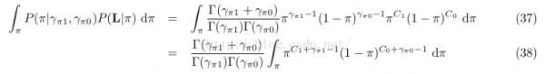
而38式后面的積分項是1個參數為C 1 + γ π1 and C 0 + γ π0的beta散布，且Beta(C 1 + γ π1 , C 0 + γ π0 )的積分為

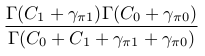
讓N = C 0 + C 1

則38式表示為：

全部文檔集的聯合散布表示（3因子式）為：

其中，N = C 0 + C 1

構建吉布斯采樣器Gibbs Sampler

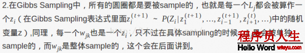
吉布斯采樣就是通過條件幾率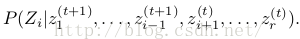給Zi1個新值

如要計算，需要計算條件散布

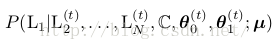
Note: There’s no superscript on the bags of words C because they’re fully observed and don’t change from iteration to iteration.

要計算θ 0，需要計算條件散布

直覺上，在每一個迭代t開始前，我們有以下當前信息：

每篇文檔的詞計數，標簽為0的文檔計數，標簽為1的文檔計數，每篇文檔確當前label，θ0 和 θ1確當前值等等。

采樣準則

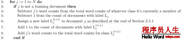
采樣label：When we want to sample the new label for document j, we temporarily remove all information (i.e. word counts and label information) about this document from that collection of information. Then we look at the conditional probability that L j = 0 given all the remaining information, and the conditional probability that L j = 1 given the same information, and we sample the new label L j (t+1) by choosing randomly according to the relative weight of those two conditional probabilities.

采樣θ：Sampling to get the new values operates according to the same principal.

2.5.1 文檔標簽的采樣

定義條件幾率

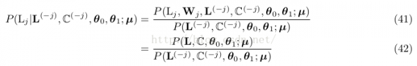
L (?j) are all the document labels except L j , and C (?j) is the set of all documents except W j .

份子是全聯合幾率散布，分母是除去Wj信息的相同的表達式，所以我們需要斟酌的只是式40的3個因子。

其實我們要做的只是斟酌除去Wj后，改變了甚么。

因子1

由于因子1僅依賴于超參數，份子分母1樣，不予斟酌，故只斟酌式40中的因子2和因子3。

因子2

式42因子2分母的計算與上1次迭代Lj是多少有關。

不過語料大小總是從N變成了N⑴，且其中1個文檔種別的計數減少1。如Lj=0，則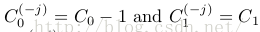，Cx只有1個有變化，這樣

let x be the class for which C x(?j)= C x ? 1，式42的因子2重寫為：

又Γ(a + 1) = aΓ(a) for all a

這樣式42的因子2簡化為：

因子3

同因子2，總有某個class對應的項沒變，也就是式42的因子3中θ 0 or θ 1有1項在份子和分母中是1樣的。

合并

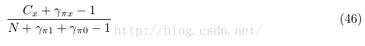
for x ∈ {0, 1}，終究合并得到采樣文檔label的的條件散布為

從式49看文檔的label是如何選擇出來的：

式49因子1：L j = x considering only the distribution of the other labels

式49因子2：is like a word distribution “fitting room.”, an indication of how well the words in W j “fit” with each of the two distributions.

前半部份其實只有Cx是變量，所以如果C0大，則P(L(t+1)j=0)的幾率就會大1點，所以下1次Lj的值就會偏向于C0，反之就會偏向于C1。而后半部份，是在判斷當前θ參數的情況下，全部文檔的likelihood更偏向于C0還是C1。

式42的條件散布采樣進程以下

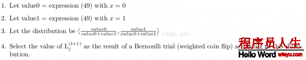
Note: 步驟3是對兩個label的幾率散布進行歸1化。

對監督數據

Using labeled documents just don’t sample L j for those documents! Always keep L j equal to the observed label.

The documents will effectively serve as “ground truth” evidence for the distributions that created them. Since we never sample for their labels, they will always contribute to the counts in (49) and (51) and will never be subtracted out.

2.5.2 θ的采樣

由于θ 0 and θ 1的散布估計是獨立的，這里我們先消去θ下標。

明顯

since we used conjugate priors, this posterior, like the prior, works out to be a Dirichlet distribution. We actually derived the full expression , but we don’t need the full expression here. All we need to do to sample a new distribution is to make another draw from a Dirichlet distribution, but this time with parameters N C x (i) + γ θi for each i in V .

define the V dimensional vector t such that each 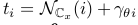（這里i下標代表V維向量t的第i個元素）:

new θ的采樣公式

從Dirichlet散布采樣的實現

sample a random vector a = <a 1 , . . . , a V> from the V -dimensional Dirichlet distribution with parameters <α 1 , . . . , α V>

最快的實現是draw V independent samples y 1 , . . . , y V from gamma distributions, each with density

然后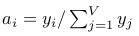（也就是正則化gamma散布的采樣）

[http://en.wikipedia.org/wiki/Dirichlet distribution]

全部樸素貝葉斯模型的吉布斯采樣框架

模型初始化

=<1, 1>   uninformed prior: uniform distribution

=<1, ..., 1>   Let γθ be a V-dimensional vector where the value of every dimension equals 1.   uninformed prior

Pick a value π by sampling from the Beta(γ π1 , γ π0 ) distribution. sample出文檔j的label為1的幾率，也就知道了文檔j的label的bernoulli幾率散布(π, 1-π)。

Then, for each j, flip a coin with success probability π, and assign label L j(0)— that is, the label of document j at the 0 th iteration – based on the outcome of the coin flip. 通過上步得到的bernoulli散布sample出文檔的label。

Similarly,you also need to initialize θ 0 and θ 1 by sampling from Dirichlet(γθ ).

模型迭代

2.5.1 文檔j標簽label的采樣公式

2.5.2 θ采樣中的（這里i下標代表V維向量t的第i個元素）

Note: lz: 如果要并行計算，特別注意的變量主要只有3個：，，

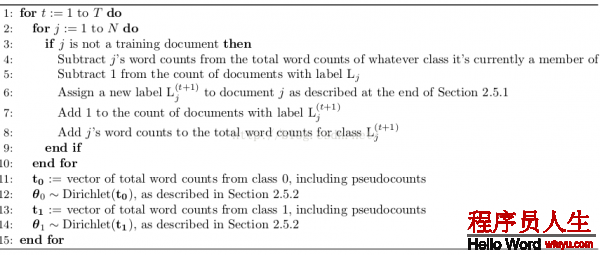
算 法中第3步好像寫錯了，應當去掉not?

Note:  as soon as a new label for L j is assigned, this changes the counts that will affect the labeling of the subsequent documents. This is, in fact, the whole principle behind a Gibbs sampler!

從吉布斯采樣中產生值

吉布斯采樣算法的初始化和采樣迭代都會產生每一個變量的值（for iterations t = 1, 2, . . . , T），In theory, the approximated value for any variable Z i can simply be obtained by calculating:

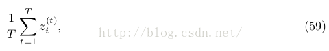
正如我們所知，吉布斯采樣迭代進入收斂階段才是穩定散布，所以1般式59加和不是從1開始，而是B + 1 through T，要拋棄t < B的采樣結果。

In this context, Jordan Boyd-Graber (personal communication) also recommends looking at Neal’s [15] discussion of likelihood as a metric of convergence.

皮皮blog

PS

1 2.6 Optional: A Note on Integrating out Continuous Parameters

In Section 3 we discuss how to actually obtain values from a Gibbs sampler, as opposed to merely watching it walk around the state space. (Which might be entertaining, but wasn’t really the point.) Our discussion includes convergence and burn-in, auto-correlation and lag, and other practical issues.

In Section 4 we conclude with pointers to other things you might find it useful to read, as well as an invitation to tell us how we could make this document more accurate or more useful.

同步圖計算并行化處理

lz的不1定正確。。。

將文檔數據分成M份，散布在M個worker節點中。

超步1：所有節點運行樸素貝葉斯吉布斯采樣算法的模型初始化部份，得到，，的初始值

超步2+：

超步開始前，主節點通過其它節點發來的改變的增量信息計算的新值，并分發給worker所有節點。（全局模型）

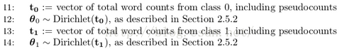
每一個節點保存有自己的信息，收到其它節點發來的改變的增量信息，主節點發來的信息

重新運行重新樸素貝葉斯吉布斯采樣算法的模型的迭代部份，計算新值（局部模型）

全部節點的數據迭代完成后計算改變的增量信息，并在超步結束后發給主節點。

burn-in階段拋棄所有節點采樣結果；收斂階段將所有節點得到的采樣結果：所有文檔的標簽值記錄下來。

全部進程進行屢次迭代，最后文檔的標簽值就是所有迭代得到的向量[標簽值]的均值偏向的標簽值。

還有1種同步圖并行計算多是這樣?

類似Spark MLlib LDA 基于GraphX實現原理，以文檔到詞作為邊，以詞頻作為邊數據，把語料庫構造成圖，把對語料庫中每篇文檔的每一個詞操作轉化為在圖中每條邊上的操作，而對邊RDD處理是GraphX中最多見的的處理方法。 

[Spark MLlib LDA 基于GraphX實現原理及源碼分析]

基于GraphX實現的Gibbs Sampling LDA，定義文檔與詞的2部圖，頂點屬性為文檔或詞所對應的topic向量計數，邊屬性為Gibbs Sampler采樣生成的新1輪topic。每輪迭代采樣生成topic，用mapReduceTriplets函數為文檔或詞累加對應topic計數。這好像是Pregel的處理方式？Pregel實現過LDA。

[基于GraphX實現的Gibbs Sampling LDA]

[Collapsed Gibbs Sampling for LDA]

[LDA中Gibbs采樣算法和并行化]

from: http://blog.csdn.net/pipisorry/article/details/51525308

ref:  Philip Resnik : GIBBS SAMPLING FOR THE UNINITIATED*

Reading Note : Gibbs Sampling for the Uninitiated