您當前位置：首頁 > php開源 > php教程 > 基于Python3 神經網絡的實現

基于Python3 神經網絡的實現

來源：程序員人生發布時間：2016-07-05 14:52:40 閱讀次數：4931次

基于Python3 神經網絡的實現

本次學習是Denny Britz（作者）的Python2神經網絡項目修改成基于Python3實現的神經網絡（本篇博文代碼完全）。重在理解原理和實現方法，部份翻譯不夠準確，可查看Python2版的原文。原文英文地址（基于Python2）

概述如何搭建開發環境

安裝Python3、安裝jupyter notebook和其他科學棧如numpy

pip install jypyter notebook
pip install numpy

生成測試數據集

# 導入需要的包
import matplotlib.pyplot as plt
import numpy as np
import sklearn
import sklearn.datasets
import sklearn.linear_model
import matplotlib

# Display plots inline and change default figure size
%matplotlib inline
matplotlib.rcParams['figure.figsize'] = (10.0, 8.0)

生成數據集

make_moons數據集生成器

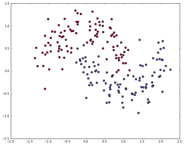
# 生成數據集并繪制出來
np.random.seed(0)
X, y = sklearn.datasets.make_moons(200, noise=0.20)
plt.scatter(X[:,0], X[:,1], s=40, c=y, cmap=plt.cm.Spectral)

<matplotlib.collections.PathCollection at 0x1e88bdda780>

這里寫圖片描述

邏輯回歸

為了證明（學習特點）這點，讓我們來訓練1個邏輯回歸分類器吧。以x軸，y軸的值為輸入，它將輸出預測的類（0或1）。為了簡單起見，這兒我們將直接使用scikit-learn里面的邏輯回歸分類器。

# 訓練邏輯回歸訓練器
clf = sklearn.linear_model.LogisticRegressionCV()
clf.fit(X, y)

LogisticRegressionCV(Cs=10, class_weight=None, cv=None, dual=False,
           fit_intercept=True, intercept_scaling=1.0, max_iter=100,
           multi_class='ovr', n_jobs=1, penalty='l2', random_state=None,
           refit=True, scoring=None, solver='lbfgs', tol=0.0001, verbose=0)

# Helper function to plot a decision boundary.
# If you don't fully understand this function don't worry, it just generates the contour plot below.
def plot_decision_boundary(pred_func):
    # Set min and max values and give it some padding
    x_min, x_max = X[:, 0].min() - .5, X[:, 0].max() + .5
    y_min, y_max = X[:, 1].min() - .5, X[:, 1].max() + .5
    h = 0.01
    # Generate a grid of points with distance h between them
    xx, yy = np.meshgrid(np.arange(x_min, x_max, h), np.arange(y_min, y_max, h))
    # Predict the function value for the whole gid
    Z = pred_func(np.c_[xx.ravel(), yy.ravel()])
    Z = Z.reshape(xx.shape)
    # Plot the contour and training examples
    plt.contourf(xx, yy, Z, cmap=plt.cm.Spectral)
    plt.scatter(X[:, 0], X[:, 1], c=y, cmap=plt.cm.Spectral)

# Plot the decision boundary
plot_decision_boundary(lambda x: clf.predict(x))
plt.title("Logistic Regression")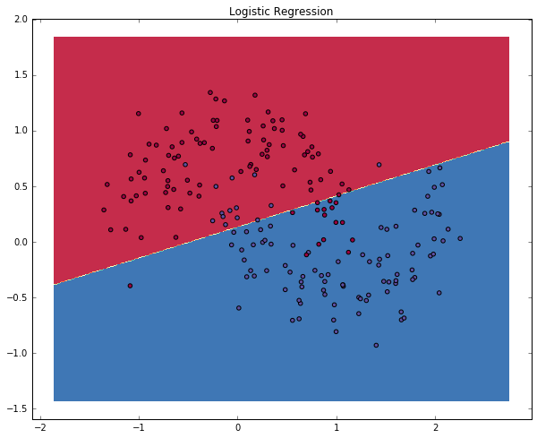

這里寫圖片描述

The graph shows the decision boundary learned by our Logistic Regression classifier. It separates the data as good as it can using a straight line, but it’s unable to capture the “moon shape” of our data.

訓練1個神經網絡

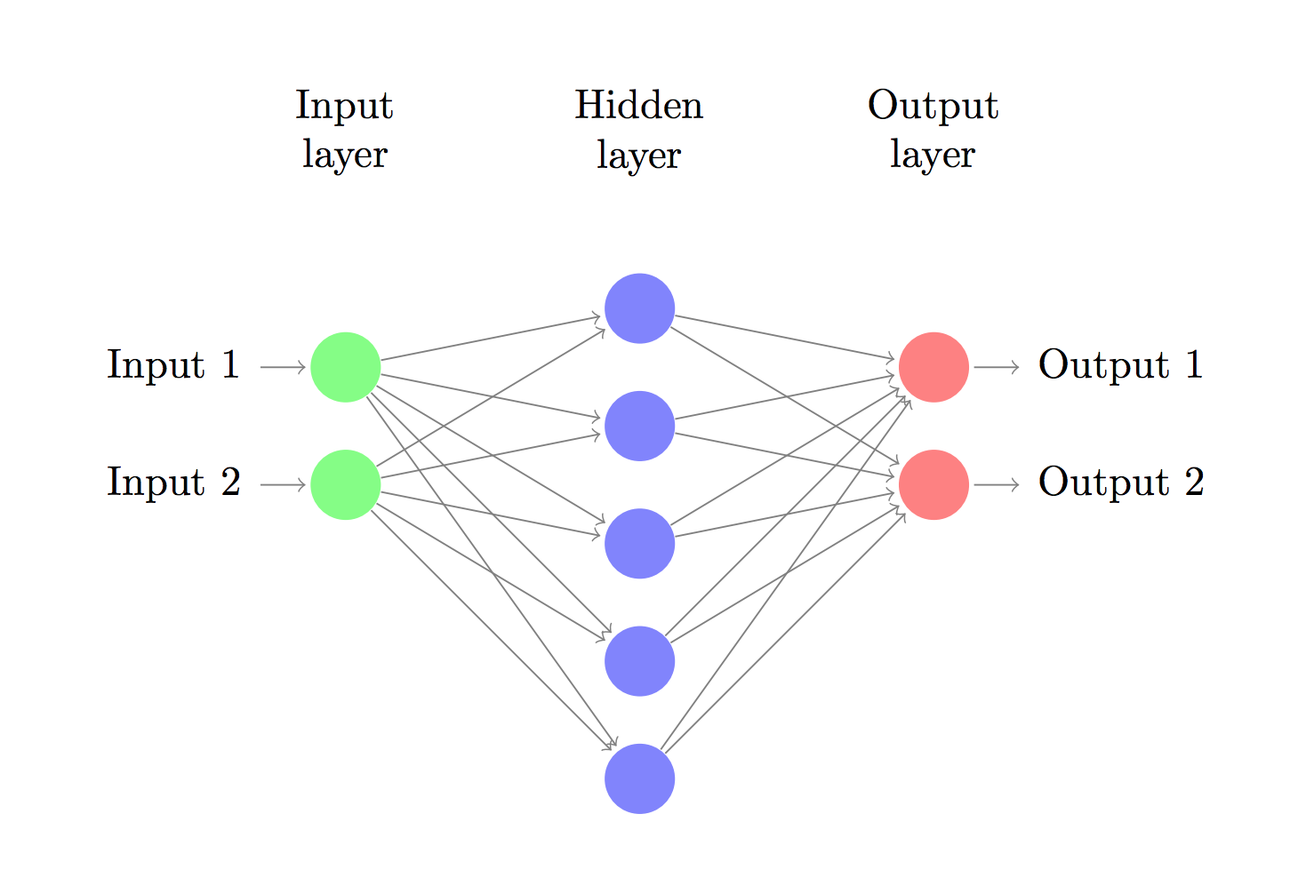
現在，我們搭建由1個輸入層，1個隱藏層，1個輸出層組成的3層神經網絡。輸入層中的節點數由數據的維度來決定，也就是2個。相應的，輸出層的節點數則是由類的數量來決定，也是2個。（由于我們只有1個預測0和1的輸出節點，所以我們只有兩類輸出，實際中，兩個輸出節點將更容易于在后期進行擴大從而取得更多種別的輸出）。以x，y坐標作為輸入，輸出的則是兩種幾率，1種是0（代表女），另外一種是1（代表男）。結果以下：

神經網絡作出預測原理

神經網絡通過前向傳播做出預測。前向傳播僅僅是做了1堆矩陣乘法并使用了我們之前定義的激活函數。如果該網絡的輸入x是2維的，那末我們可以通過以下方法來計算其預測值：

z 1 a 1 z 2 a 2 = x W 1 + b 1 = tanh (z 1) = a 1 W 2 + b 2 = y^= s o f t m a x (z 2)

zi is the input of layer i and ai is the output of layer i after applying the activation function. W1,b1,W2,b2 are parameters of our network, which we need to learn from our training data. You can think of them as matrices transforming data between layers of the network. Looking at the matrix multiplications above we can figure out the dimensionality of these matrices. If we use 500 nodes for our hidden layer then W1∈R2×500, b1∈R500, W2∈R500×2, b2∈R2. Now you see why we have more parameters if we increase the size of the hidden layer.

研究參數

Learning the parameters for our network means finding parameters (W1,b1,W2,b2) that minimize the error on our training data. But how do we define the error? We call the function that measures our error the loss function. A common choice with the softmax output is the cross-entropy loss. If we have N training examples and C classes then the loss for our prediction y^ with respect to the true labels y is given by:

L (y, y^) = ? 1 N \sum n \in N \sum i \in C y n, i log y^n, i

The formula looks complicated, but all it really does is sum over our training examples and add to the loss if we predicted the incorrect class. So, the further away y (the correct labels) and y^ (our predictions) are, the greater our loss will be.

Remember that our goal is to find the parameters that minimize our loss function. We can use gradient descent to find its minimum. I will implement the most vanilla version of gradient descent, also called batch gradient descent with a fixed learning rate. Variations such as SGD (stochastic gradient descent) or minibatch gradient descent typically perform better in practice. So if you are serious you’ll want to use one of these, and ideally you would also decay the learning rate over time.

As an input, gradient descent needs the gradients (vector of derivatives) of the loss function with respect to our parameters: ?L?W1 生活不易，碼農辛苦
如果您覺得本網站對您的學習有所幫助,可以手機掃描二維碼進行捐贈
程序員人生